Sept./24/2013 (Mw 7.7), Balochistan, Pakistan
Location of Epicenter |
Overview
|
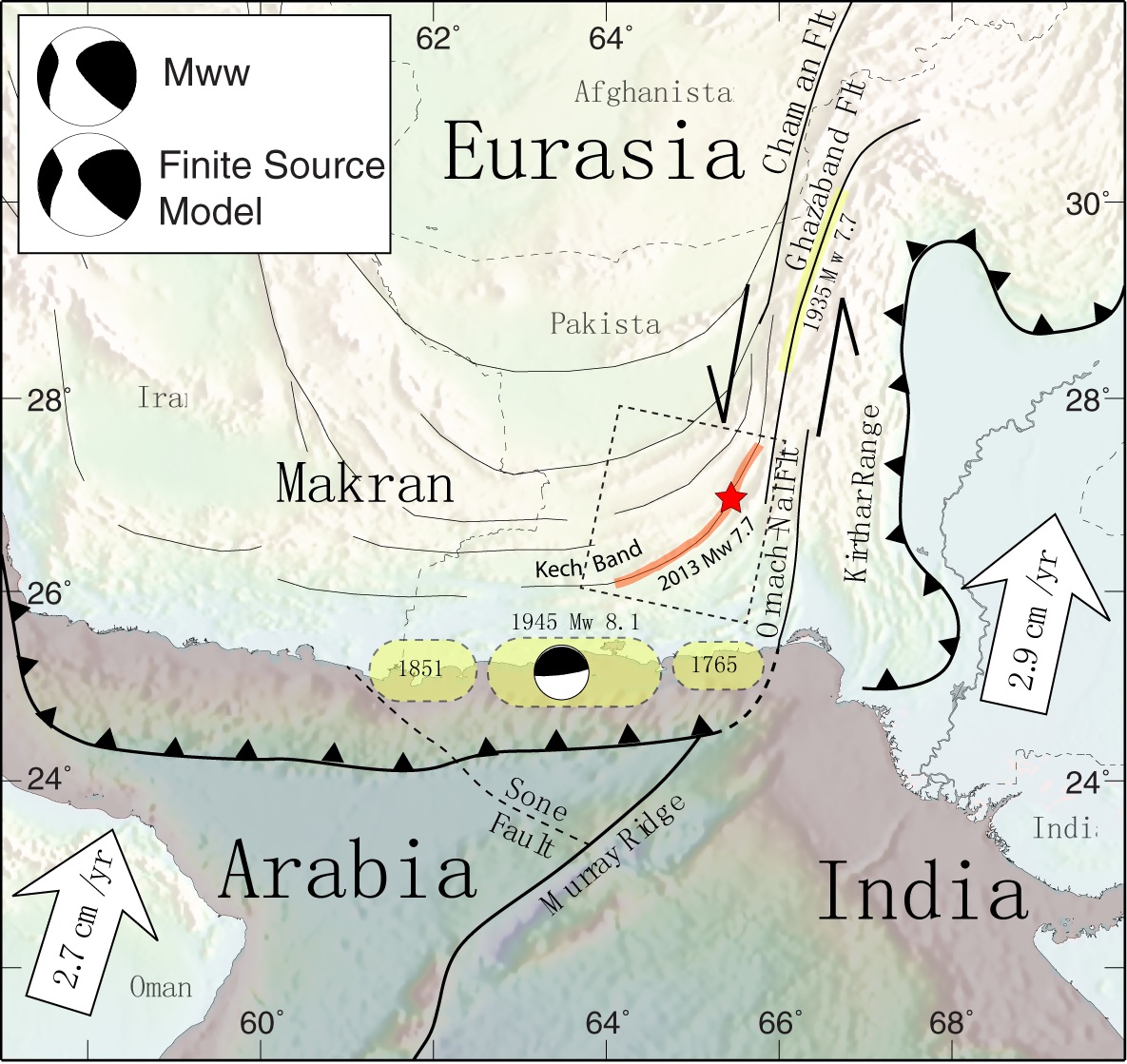
Seismotectonic setting of the September 24, 2013, Mw 7.7 Balochistan earthquake. The location of the epicenter, red star shows that the earthquake nucleated at the southern tip of the Chaman fault, the major left-lateral strike-slip fault accommodating the northward motion of India relative to Eurasia. The curved trace of the surface rupture shows that the earthquake propagated along a restraining fault bend within the Makran accretionnary prism. The box shows the footprint of map view for the slip model. The W-phase moment tensor determined (inset) shows purely strike motion on the fault plane sub-parallel to the observed fault trace. The 10% non-double component is consistent with the curved geometry of the fault trace. The moment tensor of the finite source model (also in inset) is nearly identical to the W-phase moment tensor. |
DATA Process and Inversion
The source model is obtained by joint inversion of optical data and GSN broadband data downloaded from the IRIS DMC. We analyzed 97 teleseismic P waveforms and 86 SH waveforms selected based upon data quality and azimuthal distribution. Waveforms are first converted to displacement by removing the instrument response and then used to constrain the slip history based on a finite fault inverse algorithm (Ji et al, 2002). The epicenter location is determined by trial-and-error, using both the static and teleseismic waveforms, which is: 26.870N 65.325E. The fault geometry is determined by static inversion using the optical data. Here we used 7 segments, see the map for location and geometry of these segments. See (Avouac et. al.2014) for more details.Data and Result:
Optical Data
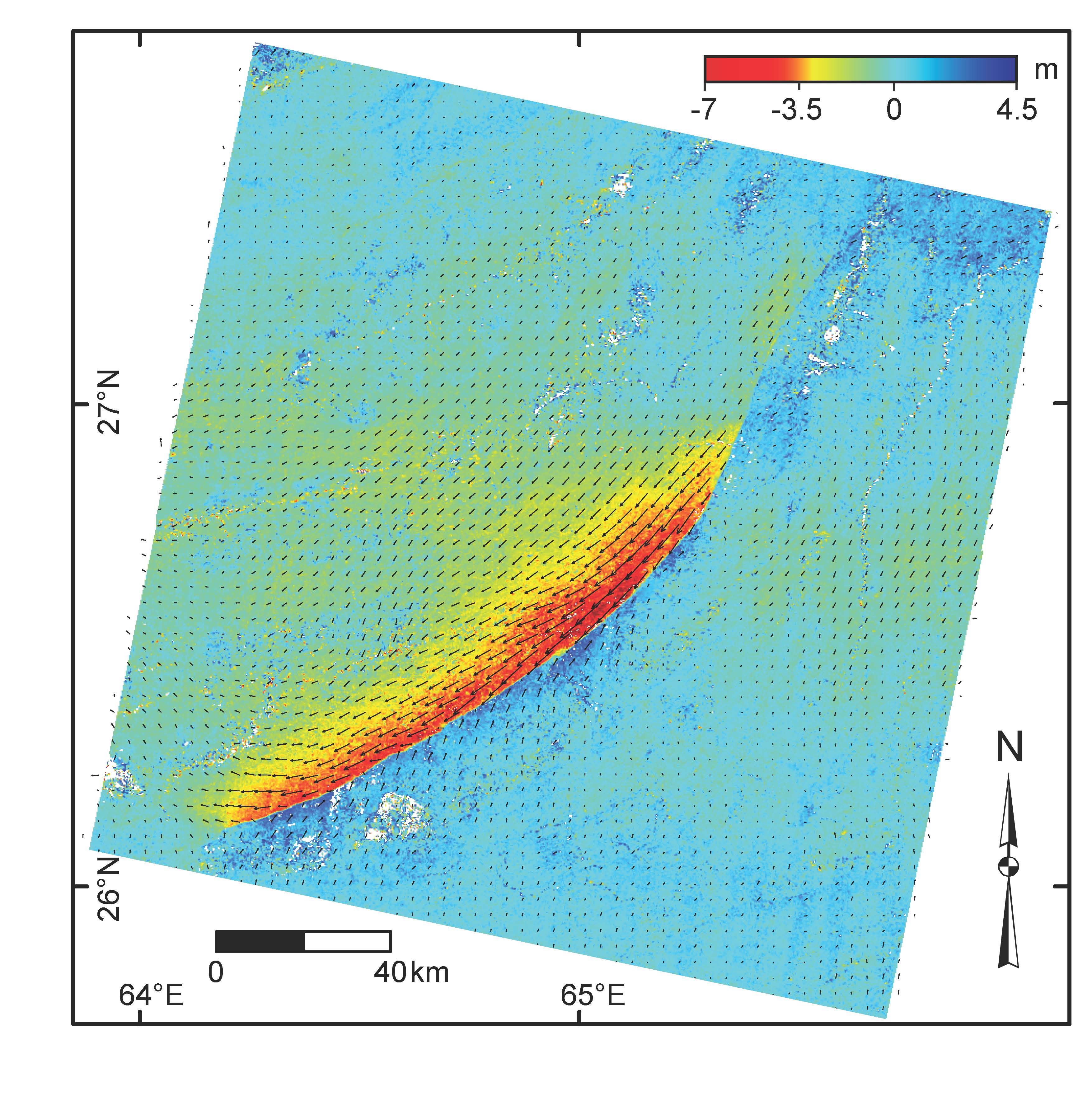
urface displacement measured from cross-correlation of optical satellite images. We used two pairs of Landsat 8 images (15m GSD), acquired on 09/10/13 and 09/26/13, which were co-registered and correlated using COSI-Corr (Leprince et al., 2007). Vector field show horizontal displacements and color shading shows the EW component of the displacement field (positive eastward) calculated with a 64x64 pixel correlation window and a 240 m Ground Sampling Distance (GSD). The 1- uncertainty on EW and NS displacement is estimated to 0.47 m and 0.60 m, respectively.
Map-view of Slip Model
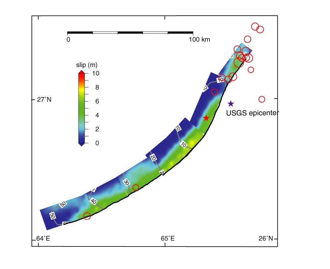
Figure 2: Finite source kinematic model. Slip distribution in map view with isochrons (in seconds) of the rupture front propagation determined from the joint inversion of the surface displacements and teleseismic waveforms. The average speed of the rupture is 3 km/s for this preferred model. Red circles show aftershocks with mb>4. over the first week following the mainshock (NEIC catalogue).
Comparison of data and synthetic seismograms
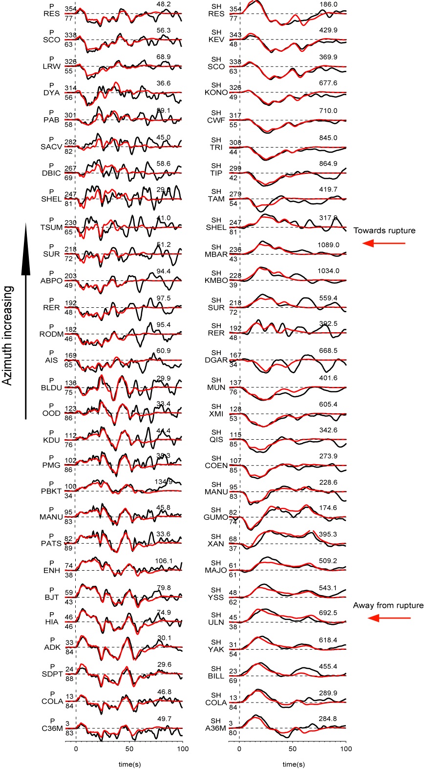
Figure 2: Representative waveform comparison of the observed (black) and modeled (red) teleseismic seismograms (in displacement). Station names are indicated to the left of the traces along with the azimuths and epicentral distances in degrees. Peak amplitude in micron of data is indicated above the end of each trace.
Station Map
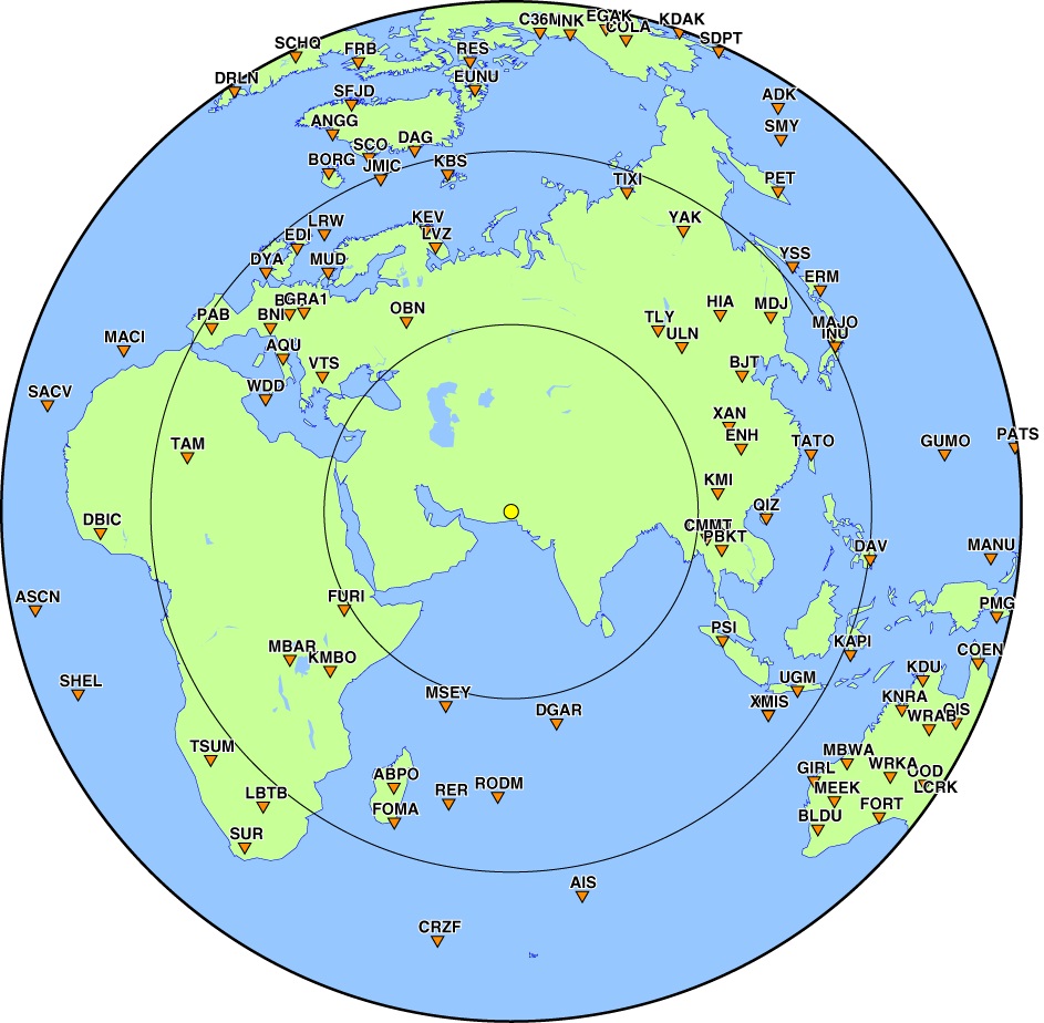
Figure 3: Teleseismic station distribution.
Moment-rate and Rupture Speed
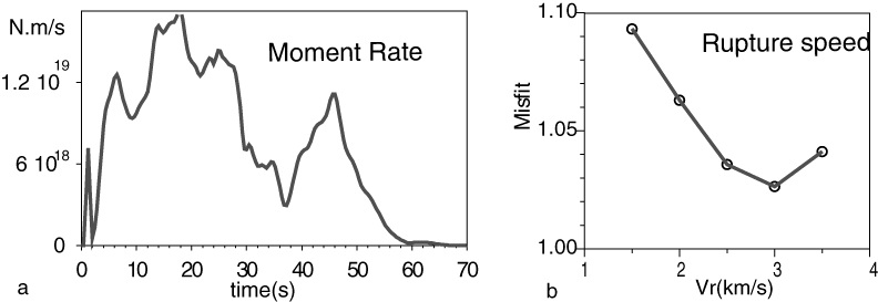
Figure 4: (a) Moment rate function corresponding to the finite source model of Figure 7. (b) Sensitivity to the rupture speed determined by running inversions with an imposed constant rupture speed. The best fitting model is obtained for a rupture speed of 3 km/s, close to the average value of our preferred model, and close to the estimated S-waves velocity in the depth range of the rupture.
Back-projection Results:
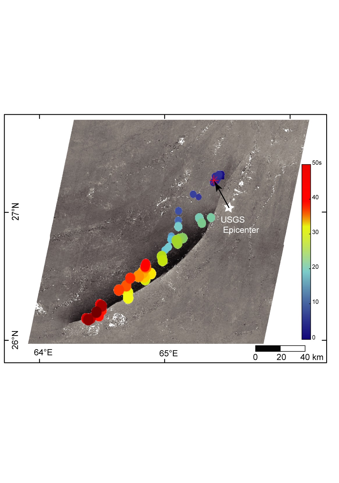
Figure 5: Rupture kinematics from backprojection of teleseismic P-waves. Rupture process imaged from back-projection of teleseismic P-waves recorded by the Japanese seismic network using the Multitaper-MUSIC array processing technique (Meng et al., 2011). Color dots show the locations of the high frequency sources (frequency band: 0.5-2 Hz). Size is proportional to the beamforming amplitude and color indicates the time of each window center relative to hypocentral time. The sliding window duration is 10 s and the first window is centered on first P waves arrival.
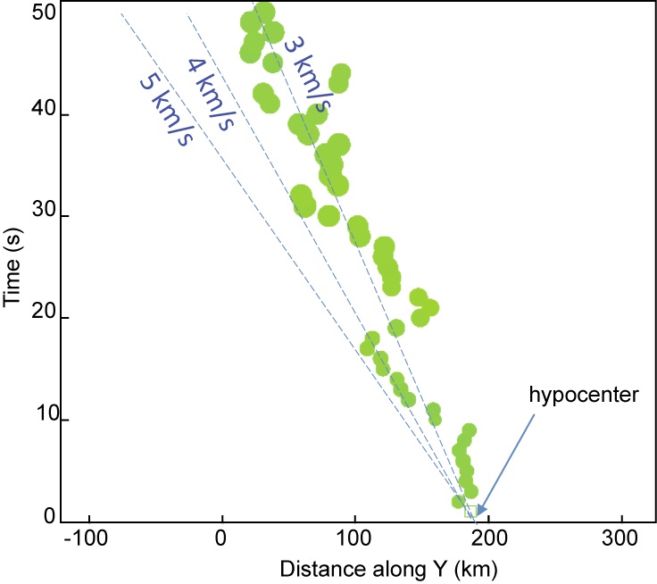
Figure 6: Timing of the high frequency sources plotted as a function of distance along the fault indicates westward unilateral rupture with average speed of about 3 km/s.
Comments:
Download
(Slip Distribution)
| SUBFAULT FORMAT | CMTSOLUTION FORMAT | SOURCE TIME FUNCTION |
References
Avouac. J-P, et al. The 2013, Mw7.7 Balochistan earthquake, energetic strike-slip reactivation of a thrust fault. EPSL, 2014, http://dx.doi.org/10.1016/j.epsl.2014.01.036Ji, C., D.J. Wald, and D.V. Helmberger, Source description of the 1999 Hector Mine, California earthquake; Part I: Wavelet domain inversion theory and resolution analysis, Bull. Seism. Soc. Am., Vol 92, No. 4. pp. 1192-1207, 2002.
Bassin, C., Laske, G. and Masters, G., The Current Limits of Resolution for Surface Wave Tomography in North America, EOS Trans AGU, 81, F897, 2000.
USGS National Earthquake Information Center: http://neic.usgs.gov
Global Seismographic Network (GSN) is a cooperative scientific facility operated jointly by the Incorporated Research Institutions for Seismology (IRIS), the United States Geological Survey (USGS), and the National Science Foundation (NSF).
‹Back to Slip Maps for Recent Large Earthquakes home page
© 2004 Tectonics Observatory :: California
Institute of Technology :: all rights reserved