Preliminary Result
07/08/15 (Mw 8.0) , Peru Earthquake
A. Ozgun Konca, Caltech
DATA Process and Inversion
We used the GSN broadband data downloaded from the IRIS DMC. We analyzed 18 teleseismic P waveforms and 19 teleseismic SH waveforms selected based upon data quality and azimuthal distribution. Waveforms are first converted to displacement by removing the instrument response and then used to constrain the slip history based on a finite fault inverse algorithm (Ji et al, 2002). We use the epicenter of the USGS (Lon.=76.509° Lat.=-13.354°). We used the Harvard CMT solution to determine strike (324°) and dip (27°). The length of fault was estimated from aftershock locations.Result
.Cross-section of slip distribution

Figure 1: The big black arrow shows the fault's strike. The colors show the slip amplitude and white arrows indicate the direction of motion of the hanging wall relative to the footwall. Contours show the rupture initiation time and the red star indicates the hypocenter location.
Comparison of data and synthetic seismograms
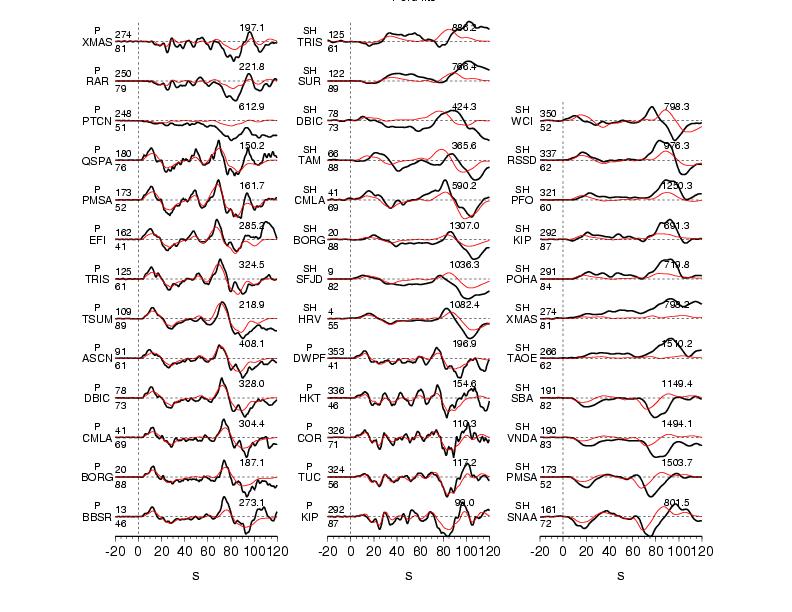
Figure 2: The Data are shown in black and the synthetic seismograms are plotted in red. Both data and synthetic seismograms are aligned on the P arrivals. The number at the end of each trace is the peak amplitude of the observation in micro-meter. The number above the beginning of each trace is the source azimuth and below it is the epicentral distance.
Map view of the slip distribution
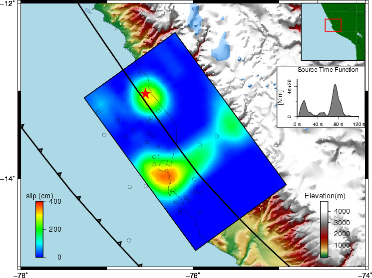
Figure 3: Surface projection of the slip distribution. The surface break obtained from geodesy is shown with black line. The measured surface offsets (black) and predictions of these offsets from seismic inversiona(red) are also shown.
Static-field
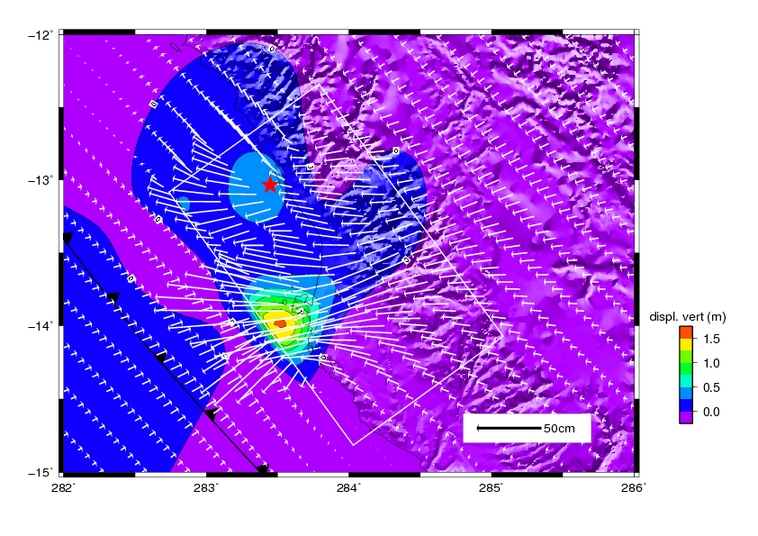
Figure 4: Static-field computed from the solution of the slip inversion. The vertical component of displacement is given by the color-scale while the arrows show the horizontal component.
Comments:
The source duration inferred from the seismic records is about 110s (Figure 2). But, because the aftershock distribution suggests a fault length of only 150 km (Figure 3), the rupture velocity is probably very slow, below 2km/s.
Download
(Slip Distribution)| SUBFAULT FORMAT | CMTSOLUTION FORMAT | SOURCE TIME FUNCTION |
References
Bassin, C., Laske, G. and Masters, G., The Current Limits of Resolution for Surface Wave Tomography in North America, EOS Trans AGU, 81, F897, 2000.Ji, C., D.J. Wald, and D.V. Helmberger, Source description of the 1999 Hector Mine, California earthquake; Part I: Wavelet domain inversion theory and resolution analysis,
GCMT project: http://www.globalcmt.org/
USGS National Earthquake Information Center: http://neic.usgs.gov
Global Seismographic Network (GSN) is a cooperative scientific facility operated jointly by the Incorporated Research Institutions for Seismology (IRIS), the United States Geological Survey (USGS), and the National Science Foundation (NSF).
‹Back to Slip Maps for Recent Large Earthquakes home page
© 2004 Tectonics Observatory :: California
Institute of Technology :: all rights reserved